2020-08-28 TSRT78 TEN1
Setup.
savefigure = @(basename) saveas(gcf(), ['figures/' basename '.png']);
rmdir('figures', 's');
mkdir('figures');
set(0, 'defaultTextInterpreter', 'latex');
set(0, 'defaultLegendInterpreter', 'latex');
set(0, 'defaultAxesTickLabelInterpreter', 'latex');
digits(4);
addpath('dsp');
1. Match spectra with windows
Since
- Longer window \(\implies\) less leakage, better frequency resolution.
- Smoother window “borders” \(\implies\) smaller side lobes, better frequency resolution.
we have
- A: 3.
- B: 1.
- C: 2.
- D: 4.
2. State space model characteristics
clear();
A = [
    1.1, 1;
    0, 0.9;
];
B = [
    1;
    1;
];
C = [
    0, 1;
];
a) Stability
tf(ss(A, B, C, 0, -1))\[ \frac{1}{z - 0.9} \]
Poles inside unit circle \(\implies\) stable, i.e. not unsable.
b) Observability
rank(obsv(A, C)) == length(A)\[ \mathrm{False} \]
The observability matrix does not have full rank \(\implies\) not observable.
c) Measurement stationarity
Since the system is stable, the statistical properties must settle into a steady state as \(k \to \infty\), i.e. yes, \(y_k\) becomes a stationary stochastic process as \(k \to \infty\).
d) State stationarity
The (unobservable) first element of \(x_n\) grows without bound as \(k \to \infty\), so no, \(x_k\) does not become as stationary process as \(k \to \infty\).
3. FIR filter characteristics
clear();
close('all');

h = [-2, -1, 0, 1, 2];

nfft = 2^10;
w = linspace(-1, +1, nfft);
a) Causality
It does not hold that \(h_n = 0, n < 0\), so no, \(h_n\) is not causal.
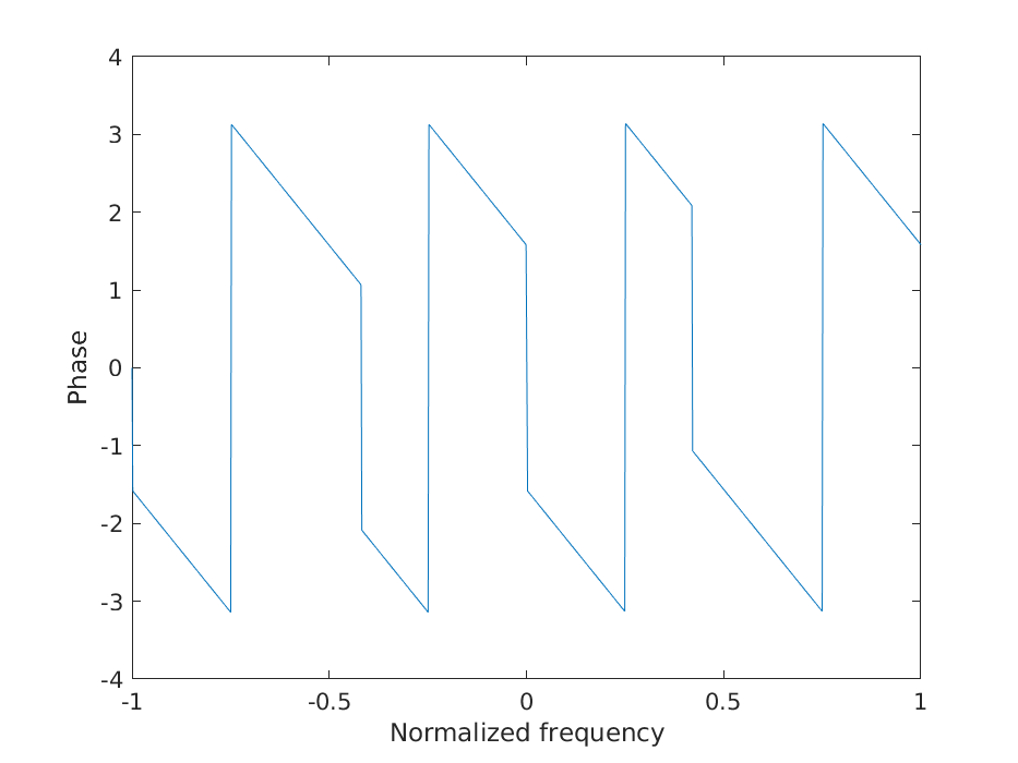
b) Phase shift
figure();
plot(w, angle(fft(h, nfft)));
xlabel('Normalized frequency');
ylabel('Phase');
savefigure('3b');
No, the filter does not have a constant phase shift.
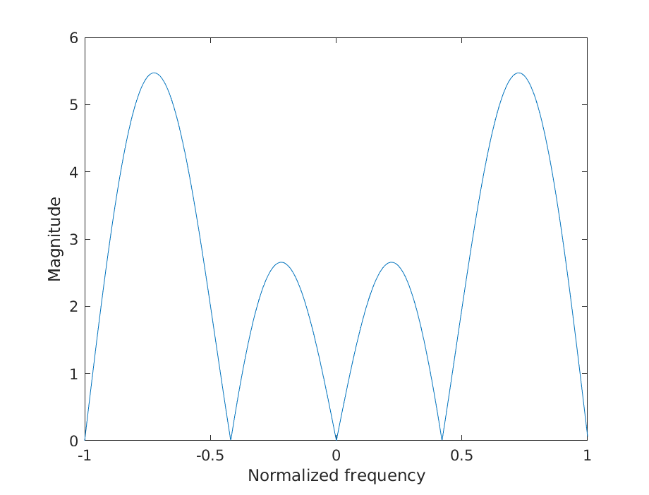
c) Filter type
figure();
plot(w, abs(fft(h, nfft)));
xlabel('Normalized frequency');
ylabel('Magnitude');
savefigure('3c');
No, the filter is not a low-pass filter.
d) Filter operation
The typical sobel filter (which is a discrete differentiation operator) is \[ f_n = [-1, 0, +1] \]
of which our \(h_n\) can be seen as a variant, so yes, the output of the filter is the derivative of the input.
4. Wiener filter from impulse response
Introduce
\[ x_n = h_n * s_n \]
clear();
close('all');

% The given variances and impulse response.
var_s = 2;
var_v = 1;
h = [2, 1, 4, 3, 1];

% Transform.
N = length(h);
H = ztrans(sum(h .* kroneckerDelta(0:N-1, sym('n'))));

% Compute spectra.
syms z;
Phi_ss = var_s;
Phi_vv = var_v;
Phi_xx = H * subs(H, z, 1/z) * Phi_ss;
Phi_yy = Phi_xx + Phi_vv;

% Perform spectral factorization.
[N, D] = numden(Phi_yy);
Nc = coeffs(N);
Dc = coeffs(D);
K = Nc(1) / Dc(1);
if length(Nc) > 3
    N = vpa(N);
end
if length(Dc) > 3
    D = vpa(D);
end
Z = solve(N);
P = solve(D);
for Z0 = Z(abs(Z) > 1)'
    K = - K * Z0;
    Z = [Z; 0];
end
for P0 = P(abs(P) > 1)'
    K = - K / P0;
    P = [P; 0];
end
Z = Z(abs(Z) < 1);
P = P(abs(P) < 1);
T = prod(z - Z) / prod(z - P);
var_e = K;

% Create and find the causal part of He by polynomial division and partial
% fraction expansion.
He = Phi_xx / (var_e * subs(T, z, 1/z));
[N, D] = numden(He / z);
[P, N, R] = poles(polynomialReduce(N, D) / D);
partfracs = R ./ (z - P) .^ N;
Hep = z * sum(partfracs(abs(P) < 1));

% Compute causal Wiener filter.
Hc = 1 / T * Hep;

% Transform.
hc = iztrans(Hc);

% Display result.
disp(vpa(simplify(hc)));
Unfortunately, the results are garbage. Hopefully this illustrates an understanding of the general methodology.
5. Linear model estimation
a) Model order and estimation
clear();
close('all');

% Load data,
load('polydata');
who();
N = length(y);

% Define model.
phi = @(x, n) x .^ (0:n-1);

% Try different orders.
nmax = 15;
for n = 1:nmax
    [th, ~, lam, ~] = sig2linmod(y, phi(x, n));
    W(n) = N * lam / (y' * y);
    Uaic(n) = W(n) * (1 + 2 * n / N);
    Ubic(n) = W(n) * (1 + n * log(N) / N);
end

% Plot results.
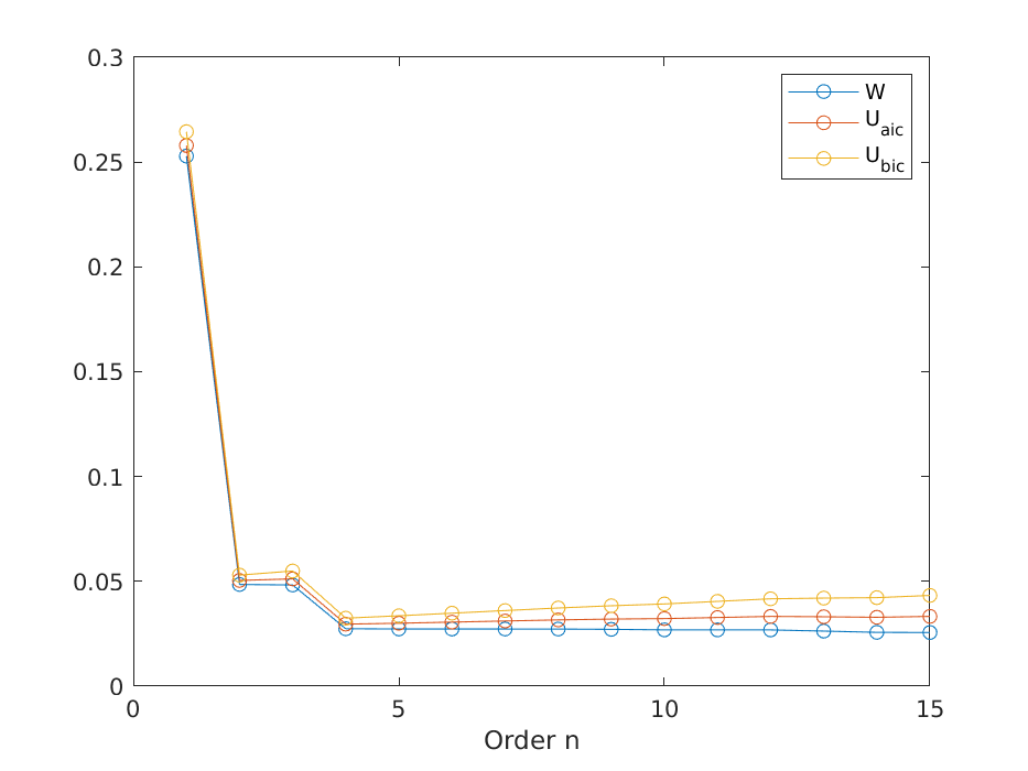
figure();
plot(1:nmax, [W', Uaic', Ubic'], '-o');
legend('W', 'U_{aic}', 'U_{bic}');
xlabel('Order n');
savefigure('5_losses');

% Determine best order.
[~, n] = min(Ubic);
disp(n);

% Create and display model.
th = sig2linmod(y, phi(x, n));
disp(th);

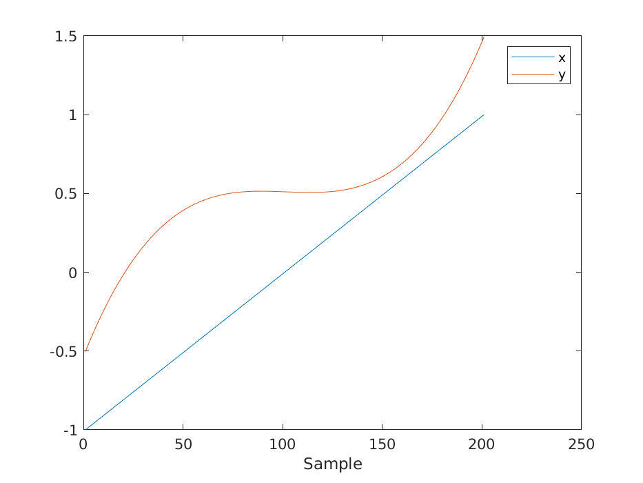
% Visualize model for special input.
x = (-1:0.01:1)';
y = phi(x, n) * th;
figure();
plot([x, y]);
legend('x', 'y');
xlabel('Sample');
savefigure('5_visualization');
Order 4 seems appropriate for which the parameters are
\[ \theta = 0.5107, -0.0477, -0.0154, 1.0461 \]
